

ML/AI, CV
Day and Night image classification using Computer Vision
Here is a classifier with no neural network, no training run and no model file. It sorts photographs into day and night, it is about fifteen lines long, and on a sensible dataset it will be right the overwhelming majority of the time.
Why bother, in the age of deep learning
Because it makes visible the thing deep learning hides.
Every image classifier, however large, does the same two jobs: reduce an image to some numbers that capture what matters, then draw a boundary through those numbers. A convolutional network learns both jobs at once from thousands of examples, which is powerful and completely opaque.
Here we do both by hand. We pick the number ourselves and we place the boundary ourselves. When it gets an image wrong you can point at exactly which of those two decisions failed, and that is a kind of understanding that is very hard to get from a network.
The pipeline
This is the standard computer vision pipeline from the What is computer vision post, and this project is about the smallest honest instance of it you can build:
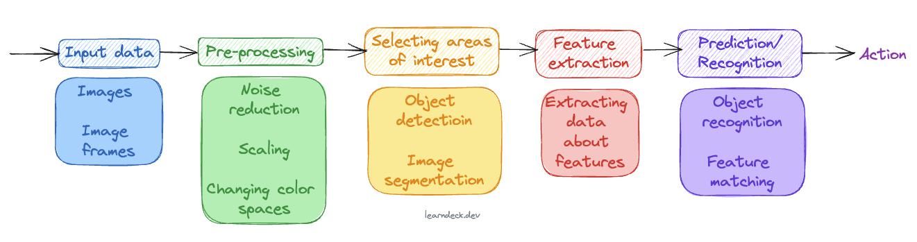
Mapped onto what we are about to write:
| Stage | What it is here |
|---|---|
| Input data | A folder of day photos and a folder of night photos |
| Pre-processing | Resize every image to one size, turn labels into numbers |
| Feature extraction | Average brightness - one float per image |
| Prediction | Is that float above a threshold |
Four steps. The interesting one is feature extraction, and it is one line.
Loading the data
Assume two folders, one of day images and one of night images:
import os
import glob

import cv2
import numpy as np
import matplotlib.pyplot as plt

%matplotlib inline

def load_dataset(image_dir):
    images = []
    for label in ('day', 'night'):
        pattern = os.path.join(image_dir, label, '*')
        for path in glob.glob(pattern):
            image = cv2.imread(path)
            if image is None:          # glob will happily hand you .DS_Store
                continue
            image = cv2.cvtColor(image, cv2.COLOR_BGR2RGB)
            images.append((image, label))
    return images

training = load_dataset('images/training')
testing  = load_dataset('images/test')

print(len(training), 'training images')
print(len(testing), 'test images')
That if image is None guard matters more than it looks. cv2.imread does not raise on a file it cannot decode - it returns None and carries on. A stray .DS_Store or thumbnail in the folder becomes a None that fails much later, somewhere confusing.
Standardising the input
Two things need to be consistent before any measurement means anything.
def standardize_input(image):
    # every image the same size, so brightness is comparable across images
    return cv2.resize(image, (1100, 600))

def encode(label):
    # day = 1, night = 0
    return 1 if label == 'day' else 0

def standardize(image_list):
    return [(standardize_input(img), encode(label)) for img, label in image_list]

standardized_training = standardize(training)
standardized_testing  = standardize(testing)
The resize is not cosmetic. We are about to take an average over pixels, and while an average is already independent of image size in principle, an inconsistent dataset makes every later step - plotting, indexing, eyeballing results - needlessly awkward. Fix the size once at the start.
Encoding day as 1 and night as 0 is a convention, but a useful one: it means accuracy is just a comparison of two integer lists, and the classifier can return the same type the labels are stored in.
The feature: average brightness
This is the whole idea. Day images are bright, night images are dark, so measure brightness and nothing else.
The HSV colour space post is what makes this easy. HSV splits colour from brightness onto separate axes, and the Value channel is brightness on its own:
def avg_brightness(rgb_image):
    hsv = cv2.cvtColor(rgb_image, cv2.COLOR_RGB2HSV)
    return np.mean(hsv[:, :, 2])       # V channel = brightness
That is the feature extractor. One line of real work.
It is worth knowing exactly what the V channel contains, because it is simpler than people assume. Value is just the largest of the three RGB channels at each pixel - V == max(R, G, B), exactly, not approximately. So "average brightness" here means: for every pixel take its strongest colour channel, then average those across the image.
That has a consequence worth carrying forward. A single vivid red pixel, (255, 0, 0), has a Value of 255 - maximum brightness - despite being quite dark to look at. Value is not perceived luminance. It is generous about anything with a strong channel, which is precisely why streetlights and neon will give us trouble later.
Choosing the threshold
Do not guess. Look at the distribution first:
day_brightness   = [avg_brightness(img) for img, lbl in standardized_training if lbl == 1]
night_brightness = [avg_brightness(img) for img, lbl in standardized_training if lbl == 0]

plt.figure(figsize=(12, 5))
plt.hist(night_brightness, bins=30, alpha=0.6, label='night')
plt.hist(day_brightness,   bins=30, alpha=0.6, label='day')
plt.xlabel('average brightness (V)')
plt.legend()

print(f'day:   {min(day_brightness):.0f} - {max(day_brightness):.0f}')
print(f'night: {min(night_brightness):.0f} - {max(night_brightness):.0f}')
You get two humps. Night piles up low, day piles up high, and there is a valley between them where the two distributions overlap a little. Put the threshold in that valley.
The overlap is the honest part of this exercise. If the two humps were cleanly separated, any threshold in the gap would do and there would be nothing to learn. They are not cleanly separated, and where you place the line inside the overlap decides which kind of mistake you make more often - calling night images day, or day images night.
Somewhere around 100 is typical for this kind of dataset, but read it off your own histogram rather than taking that number on trust.
The classifier
THRESHOLD = 100

def estimate_label(rgb_image, threshold=THRESHOLD):
    return 1 if avg_brightness(rgb_image) > threshold else 0
That is the model. Two lines, one parameter, and that parameter was set by a human looking at a chart.
Measuring accuracy
def get_misclassified(test_images):
    misclassified = []
    for image, true_label in test_images:
        predicted = estimate_label(image)
        if predicted != true_label:
            misclassified.append((image, predicted, true_label))
    return misclassified

misclassified = get_misclassified(standardized_testing)

total = len(standardized_testing)
accuracy = (total - len(misclassified)) / total
print(f'Accuracy: {accuracy:.3f}')
print(f'Misclassified: {len(misclassified)} out of {total}')
Two things about this that are habits worth forming.
Evaluate on images the threshold never saw. The histogram was plotted from the training set; accuracy is measured on the test set. It feels excessive when the "model" is a single number, but that single number was fitted to data, and a number fitted to data will always look better on that data.
Keep the failures, not just the count. get_misclassified returns the images themselves. The accuracy figure tells you how much is wrong; only the images tell you what is wrong, and that is the part you can act on.
Looking at what it gets wrong
This is the most valuable section of the project, and the one easiest to skip.
for image, predicted, true_label in misclassified:
    plt.figure()
    plt.title(f'predicted {predicted}, actually {true_label} '
              f'- brightness {avg_brightness(image):.1f}')
    plt.imshow(image)
The mistakes are not random. They fall into recognisable groups, and each one is telling you something specific about the feature:
- Night images called day. City scenes with floodlights, illuminated signs, headlight glare. Remember that Value takes the maximum channel - a bright sign is at 255 in Value regardless of colour, and enough of them drags the average over the line.
- Day images called night. Heavy overcast, storms, deep shade, photos taken indoors looking out. Genuinely dark daytime.
- Dusk and dawn, both directions. These are not really failures of the classifier. The label itself is arguable, and no threshold resolves an ambiguity that exists in the ground truth.
That last category matters. When you find your model failing on cases where two reasonable people would disagree about the correct answer, you have hit the ceiling of the problem as posed, not a bug in your code. More features will not fix it. A better dataset definition might.
Where this approach stops working
Being clear about the limits is the point of building the simple thing first:
- One feature means one axis. Everything the classifier knows is a single number. Two images with the same average brightness are indistinguishable to it, whatever else is in them.
- The threshold is fitted to this dataset. Photos from a different camera, city or climate will sit differently, and the number needs re-picking.
- It does not generalise to a third class. Adding "dusk" is not a matter of another threshold, because dusk is not simply "between" day and night in brightness - overcast noon lands there too.
The natural next step is a second feature - a colour one, since night lighting is heavily orange while daylight is broadly neutral. Average saturation, or the fraction of pixels in a warm hue band, would separate a floodlit car park from an overcast afternoon in a way brightness alone cannot. Then you have two numbers, and a line through a plane instead of a point on an axis. That is the same idea, one dimension up, and it is the road that leads to learned classifiers.
Things that will bite you
cv2.imreadreturnsNoneon failure, it does not raise. Guard the load, or a hidden file will crash you somewhere unrelated.- Never sum a
uint8array into auint8accumulator.v.sum(dtype=np.uint8)returns0on a typical image - it wraps round hundreds of times, silently.np.meanand a plainnp.sumare safe, because numpy promotes to a wider type for you. - Value is
max(R, G, B), not perceived brightness. A saturated red pixel scores 255. If you want something closer to how bright a scene looks, convert to greyscale withcv2.COLOR_RGB2GRAY, which weights the channels for human vision instead. - Standardise before measuring. Comparing features across images of different sizes and formats will eventually produce a bug you spend an afternoon on.
- Do not tune the threshold against the test set. The moment you nudge it to fix a test failure, your accuracy number stops meaning anything.